Smart Calorie Burn v2

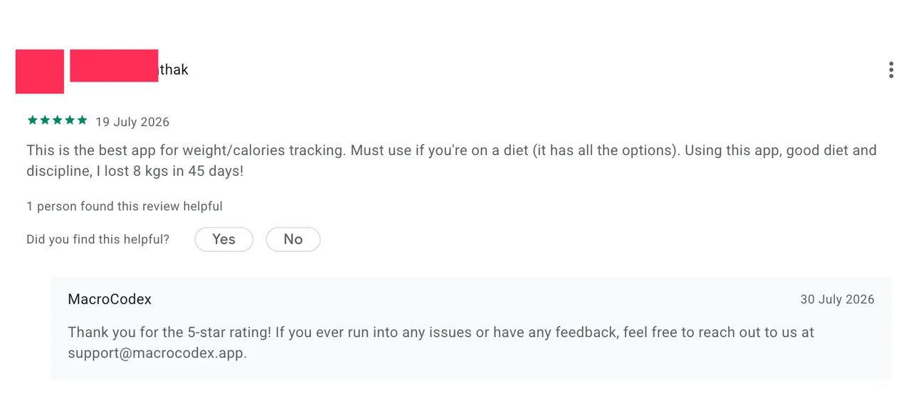
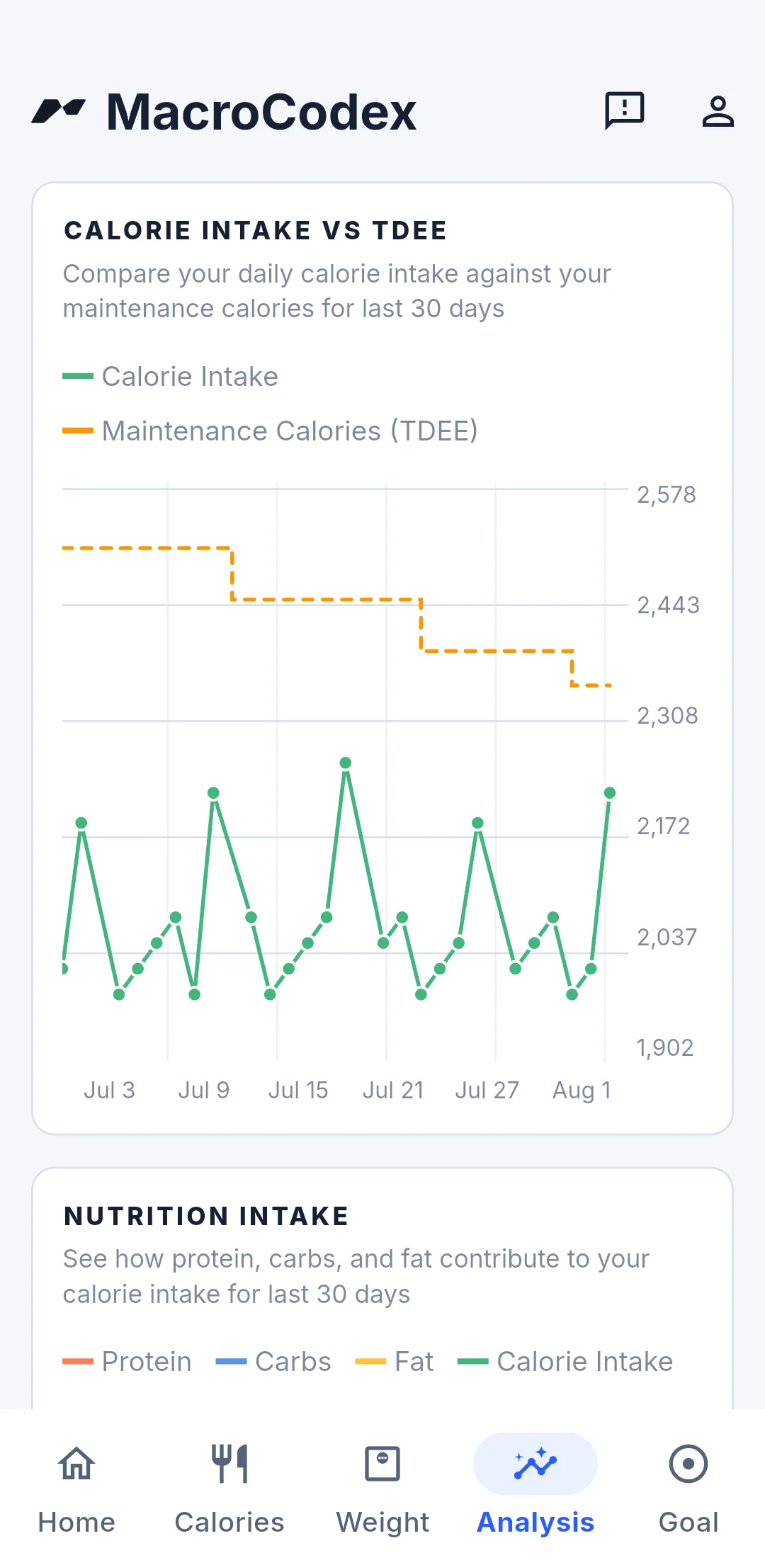
Many people ask, "How is MacroCodex, a completely free (subscription-free, ad-free) app, able to provide guaranteed weight loss or weight gain within 2-5 weeks when many coaches or dieticians fail to do so?". The answer is Smart Calorie Burn v2, the algorithm at the heart of MacroCodex. It is responsive, stable, accurate, and resilient to missing data, while accounting for temporary water weight fluctuations caused by hormonal changes, creatine use, sodium levels, carb induced glycogen swings, the menstrual cycle, stress hormones, and fluid retention.

Background and Physiological Foundations

Problem

It all started from a simple question

How much must a person eat to lose or gain X kg or Y lb of bodyweight?

Simple idea

If you ask a random layman on the street, "How do I lose or gain weight?", they'll tell you to eat less to lose weight and eat more to gain weight; the only thing that is left is to define what is "more" and what is "less".

The amount of energy the body burns in 24 hours is called Total Daily Energy Expenditure (TDEE).

The amount of calories consumed from food can be measured. Let's call this Daily Energy Intake (DEI).

If a person consistently eats more calories than they expend, some of that excess energy is stored in the body, primarily as fat and other tissue, resulting in bodyweight gain.

If a person consistently eats fewer calories than they expend, stored body energy must be used, resulting in bodyweight loss.

---

Surplus and Deficit

Define the daily energy balance as:

$$EB = \text{Daily Energy Intake} - \text{TDEE}$$

This signed quantity gives both the direction and magnitude of the imbalance:

$$\begin{aligned} EB &> 0 &&\Rightarrow\text{ energy surplus} \\ EB &< 0 &&\Rightarrow\text{ energy deficit} \\ EB &= 0 &&\Rightarrow\text{ energy balance} \end{aligned}$$

Over a period of $n$ days, the cumulative energy imbalance is:

$$\Delta E = \sum_{t=1}^{n} EB_t$$

If the cumulative balance is positive, the body must, on average, store energy; if it is negative, it must, on average, release stored energy. Thus:

$$\begin{aligned} \Delta E &> 0 &&\Rightarrow\text{ expected bodyweight gain over time} \\ \Delta E &< 0 &&\Rightarrow\text{ expected bodyweight loss over time} \end{aligned}$$

The expected magnitude of tissue-weight change is approximately related to the magnitude of the cumulative imbalance:

$$\Delta W \approx \frac{\Delta E}{D}$$

where $\Delta W$ is bodyweight change (positive for gain and negative for loss), $\Delta E$ is cumulative energy imbalance, and $D$ is the effective energy density of the weight change. Therefore, a larger sustained surplus tends to produce faster gain, and a larger sustained deficit tends to produce faster loss.

This is an approximation, not a fixed calorie-to-weight conversion: $D$ changes with the mix of fat, lean tissue, glycogen, and water, and short-term scale weight can move independently of tissue energy balance.

---

From Energy Balance to a Calorie Target

If we knew both:

1. Daily calorie intake, and
2. Total Daily Energy Expenditure

then answering:

"How many calories should this person eat?"

would become relatively straightforward.

For example, suppose someone wants to lose 1 lb per week.

If we knew the amount of energy corresponding to 1 lb of weight loss, we could calculate the required average daily deficit:

$$\text{Required Daily Deficit} = \frac{\text{Energy required for 1 lb loss}}{7}$$

Then:

$$\text{Target Calorie Intake} = \text{TDEE} - \text{Required Daily Deficit}$$

Similarly, for weight gain:

$$\text{Target Calorie Intake} = \text{TDEE} + \text{Required Daily Surplus}$$

Bodyweight can be measured.

Daily calorie intake can be estimated using calorie trackers.

Therefore, the major unknown is:

$$\boxed{\text{TDEE}}$$

But there is another unknown hidden inside the problem:

How much energy corresponds to a given amount of bodyweight gain or loss?

If we know this relationship, changes in bodyweight combined with measured calorie intake can also tell us something about the person's TDEE.

Conceptually:

$$\text{Weight Change} \approx \frac{\text{Energy Imbalance}} {\text{Energy Density of Weight Change}}$$

Rearranging:

$$\text{Energy Imbalance} \approx \text{Weight Change} \times \text{Energy Density}$$

and therefore, approximately:

$$\overline{\text{TDEE}} \approx \overline{\text{Calorie Intake}} - \frac{ \Delta W\times D }{\Delta t}$$

where the bars denote daily averages over the observation interval, $\Delta t$ is the interval length in days, $\Delta W$ is total weight change over that interval, and $D$ is the effective energy density in kcal/kg. Weight gain is positive and weight loss is negative. This time term is essential: $\Delta W\times D$ is a cumulative energy change in kcal, whereas TDEE and average calorie intake are rates in kcal/day.

This gives us the basic idea behind estimating energy expenditure from observed calorie intake and bodyweight change.

But first, we need to understand the energy density of bodyweight change.

---

Subproblem 1: Energy Required for Weight Change

How much calorie surplus or deficit is required to lose or gain 1 kg or 1 lb of bodyweight?

Max Wishnofsky — 1958

The famous "1 lb = 3,500 kcal" rule traces primarily to physician Max Wishnofsky, especially his 1958 paper Caloric Equivalents of Gained or Lost Weight in the American Journal of Clinical Nutrition.

The reasoning was based largely on the energy density of human adipose tissue.

Wishnofsky's derivation treated pure triglyceride as containing approximately:

$$9.4\text{ kcal/g}$$

But human adipose tissue is not 100% triglyceride. It also contains water, protein, connective tissue, and other components.

Wishnofsky used earlier chemical-analysis evidence suggesting adipose tissue was approximately 87% fat. These are historical model assumptions, not universal measurements of every person's adipose tissue (Thomas et al., 2014).

Therefore:

$$1\text{ lb}\approx454g$$ $$454\times0.87\approx395g\text{ lipid}$$

Using approximately 9.5 kcal/g:

$$395\times9.5\approx3750\text{ kcal}$$

After reviewing weight-loss studies and making assumptions about the composition of lost tissue, Wishnofsky arrived at the practical approximation:

$$\boxed{ 1\text{ lb bodyweight} \approx 3500\text{ kcal} }$$

Since:

$$1\text{ kg}\approx2.2046\text{ lb}$$

then:

$$3500\times2.2046 \approx 7716\text{ kcal/kg}$$

This became the familiar:

$$\boxed{ 7700\text{ kcal/kg} }$$

rule.

---

Limitations of Wishnofsky’s Rule

Wishnofsky's number was not originally meant to imply that every pound appearing or disappearing on the scale always corresponds to exactly 3,500 kcal.

It can work reasonably well as an approximation of the energy content of predominantly fat-tissue loss under certain conditions.

The problem occurs when it is turned into a fixed linear prediction such as:

$$500\text{ kcal/day deficit} \times7 = 3500\text{ kcal}$$

therefore:

$$1\text{ lb/week forever}$$

Human bodyweight does not behave this way.

Weight lost can consist of varying amounts of:

• fat mass,
• fat-free mass,
• glycogen,
• associated water,
• and other body components.

Additionally, energy expenditure changes as bodyweight changes.

Therefore, the relationship between cumulative calorie deficit and bodyweight change is not perfectly constant.

---

Forbes — 1970s–1980s

Gilbert Forbes made a major advance by studying how changes in bodyweight are partitioned between (Forbes, 1987):

• Fat Mass (FM)
• Fat-Free Mass (FFM)

The important realization was that the fraction of lost weight coming from fat-free mass is not constant.

It depends strongly on the person's existing body composition.

In simplified terms:

$$\text{higher body fat} \rightarrow \text{greater fraction of loss from FM}$$

while:

$$\text{lower body fat} \rightarrow \text{greater fraction of loss from FFM}$$

This matters because fat mass and fat-free mass have very different energy densities.

A useful approximation used in Hall's adult bodyweight model is:

$$1\text{ kg FM} \approx 9400\text{ kcal}$$

while:

$$1\text{ kg FFM} \approx 1800\text{ kcal}$$

These are rounded forms of $39.5\text{ MJ/kg}$ for fat and $7.6\text{ MJ/kg}$ for modeled lean-tissue change, respectively (Hall et al., 2011, web appendix). The lean-tissue value should not be applied to arbitrary short-term changes in scale weight or conventionally measured FFM, because those can include water and glycogen shifts.

Therefore, one kilogram of bodyweight loss does not have a universal energy value.

If the fraction of lost weight coming from fat mass is $f_{\mathrm{FM}}$, then approximately:

$$E_{\text{kg}} = 9400f_{FM} + 1800f_{FFM}$$

where:

$$f_{FM}+f_{FFM}=1$$

Forbes' work primarily predicts this partitioning from the person's adiposity/body composition.

This means:

$$\boxed{ \text{kcal required per kg of weight change is not constant} }$$

Limitations of the Forbes Model

The Forbes relationship provides an important physiological improvement over assuming that every kilogram of bodyweight change has the same energy density.

However, it does not mean that body fat alone completely determines how much fat mass and fat-free mass a person will lose.

Forbes' relationship primarily describes the expected relationship between existing body fat and the partitioning of subsequent bodyweight change.

In real-world weight loss, this partition can also be affected by the conditions under which the weight is lost.

Two people with similar body composition and the same amount of weight loss may not necessarily lose the same proportions of fat mass and fat-free mass.

Protein Intake

Dietary protein influences the preservation of lean tissue during an energy deficit.

Higher protein intake during calorie restriction has been shown to reduce the loss of lean body mass compared with lower protein intake under some conditions, particularly when combined with intensive exercise. For example, a randomized trial compared 2.4 with 1.2 g protein/kg/day during a marked deficit and intensive training (Longland et al., 2016).

Therefore:

$$\text{Protein Intake} \uparrow$$

can generally shift weight loss toward:

$$\text{FM loss} \uparrow$$

relative to:

$$\text{FFM loss} \downarrow$$

for the same amount of total bodyweight lost.

This becomes particularly important in leaner individuals, where Forbes already predicts a greater risk of losing fat-free mass.

---

Resistance Training

Resistance training provides another strong signal for retaining skeletal muscle during an energy deficit.

A person who continues progressive resistance training during weight loss can preserve more lean mass than an otherwise similar person losing the same amount of weight without resistance training. One randomized trial comparing diet alone with diet plus resistance exercise found preservation of lean bodyweight in the resistance-training group (Bryner et al., 1999).

Therefore:

$$\text{Resistance Training} \longrightarrow \text{greater FFM preservation}$$

and consequently:

$$\text{greater fraction of weight loss from FM}$$

under many dieting conditions.

Protein intake and resistance training can also interact.

Adequate protein provides the substrate required for maintaining muscle protein, while resistance exercise provides a strong stimulus for maintaining or increasing muscle tissue.

---

Why This Matters for Energy Density

This does not merely affect body composition.

It also changes the energy density of the observed weight loss.

Recall:

$$E_{\text{kg}} \approx 9400f_{FM} + 1800f_{FFM}$$

Consider two people who each lose 1 kg.

If Person A loses:

$$90\%\ \text{FM} + 10\%\ \text{FFM}$$

then:

$$E_{\text{kg}} = 0.90(9400) + 0.10(1800)$$ $$E_{\text{kg}} \approx 8640\text{ kcal/kg}$$

But if Person B loses:

$$70\%\ \text{FM} + 30\%\ \text{FFM}$$

then:

$$E_{\text{kg}} = 0.70(9400) + 0.30(1800)$$ $$E_{\text{kg}} \approx 7120\text{ kcal/kg}$$

Both people lost exactly:

$$1\text{ kg}$$

but the underlying energy deficits associated with that loss could be substantially different.

Therefore, if Smart Calorie Burn estimates average TDEE over an interval from:

$$\overline{\text{TDEE}} \approx \overline{I} - \frac{\Delta W\times E_{\text{kg}}}{\Delta t}$$

then an incorrect estimate of FM/FFM partition directly creates an error in estimated TDEE.

---

Extending Forbes for Our Use Case

Forbes gives us an important baseline:

$$f_{FM} = f(\text{adiposity})$$

But for an adaptive calorie algorithm, a more realistic conceptual model would be:

$$f_{FM} = f( \text{adiposity}, \text{protein intake}, \text{resistance training}, \text{deficit severity}, \text{rate of weight loss}, \ldots )$$

The exact contribution of each variable is difficult to estimate perfectly for an individual.

The purpose therefore should not necessarily be to build a perfect physiological body-composition model.

Instead, Forbes can provide a baseline prior for expected FM/FFM partition, which can then be adjusted when relevant information is available.

For example:

$$\text{Forbes Prediction} \xrightarrow[\text{Resistance Training}]{\text{Protein Intake}} \text{Adjusted Expected FM/FFM Partition} \longrightarrow \text{Adjusted kcal/kg}$$

This adjusted energy-density estimate can then be used by the adaptive TDEE algorithm.

The important lesson is therefore:

$$\boxed{\text{Forbes is a baseline model of tissue partitioning, not a complete model}}$$

Body composition matters, but the conditions under which weight is lost also influence the composition of that weight loss.

---

Kevin Hall — 2000s

Researchers including Kevin Hall extended this idea into mathematical energy-balance models (Hall, 2008).

Hall's 2008 work explicitly asked:

What is the required energy deficit per unit of weight loss?

Instead of assuming:

$$7700\text{ kcal/kg}$$

for everyone, the energy deficit associated with weight loss can be related to the changing proportions of fat mass and fat-free mass:

$$\boxed{ E_{\text{kg}} \approx 9400f_{FM} + 1800f_{FFM} }$$

Since $f_{\mathrm{FM}}$ and $f_{\mathrm{FFM}}$ can change as the person loses weight, the effective energy density of bodyweight loss can also change over time.

So the first major lesson from the development after Wishnofsky is:

$$\boxed{ \text{Energy density of bodyweight change is dynamic} }$$

---

Hall and Chow — 2008–2011

Hall, Chow, and colleagues then developed mathematical models in which:

• calorie intake,
• energy expenditure,
• fat mass,
• fat-free mass,
• and bodyweight

interact continuously over time.

This showed that bodyweight change should be treated as a dynamic system, rather than repeatedly applying the 3,500 kcal rule.

The landmark practical treatment was Hall et al.'s 2011 paper:

Quantification of the Effect of Energy Imbalance on Bodyweight.

The important idea was that the person's energy deficit does not remain constant simply because their calorie intake remains constant.

For example, suppose:

$$TDEE_{initial}=2500$$

and calorie intake is:

$$2000$$

Initially:

$$Deficit=500\text{ kcal/day}$$

But after losing weight, the person is smaller.

A smaller body generally requires less energy both at rest and during movement.

Their TDEE might eventually become:

$$2300$$

while intake remains:

$$2000$$

The actual deficit has therefore fallen to:

$$300\text{ kcal/day}$$

Later it may fall further.

So:

$$\boxed{ \text{A fixed calorie intake does not create a fixed energy deficit} }$$

---

Lessons From Previous Work

By the 2010s, researchers such as Thomas, Hall, Chow and others had demonstrated clearly why the conventional 3,500 kcal rule substantially overpredicts long-term weight loss when used as a linear forecasting model.

The important distinction is that:

$$3500\text{ kcal/lb}$$

is not completely meaningless.

The problem is assuming that:

1. every unit of bodyweight always has the same energy density, and
2. the person's energy expenditure remains unchanged throughout the intervention.

From the work up to this point, we can establish two major principles.

---

Principle 1: Energy Density of Weight Change Differs

One kilogram of bodyweight loss is not one kilogram of pure fat.

Weight change can contain varying proportions of:

$$FM$$

and:

$$FFM$$

and these tissues have very different energy densities.

Therefore:

$$\boxed{ \text{kcal/kg weight change varies between people and over time} }$$

The Forbes relationship provides an important physiological foundation for modeling this.

---

Principle 2: Energy Expenditure Changes as Bodyweight Changes

Some reduction in expenditure occurs simply because the person has become smaller.

Suppose:

$$TDEE_{before}=2500$$

After losing 10 kg, their new body composition might predict:

$$TDEE_{predicted}=2300$$

This reduction is not necessarily metabolic adaptation.

The person now has:

• less tissue to maintain,
• less body mass to move,
• potentially different thermic costs,
• and different energy requirements.

Therefore, some reduction in TDEE is an expected consequence of weight loss.

But this is not the entire story.

---

Leibel, Rosenbaum and Hirsch — 1995

Rudolph Leibel, Michael Rosenbaum and Jules Hirsch demonstrated an additional phenomenon.

After substantial weight loss, measured energy expenditure can fall below what would be expected simply from the person's new body size and composition.

For example:

$$TDEE_{before}=2500$$

After weight loss, the person's new body composition might predict:

$$TDEE_{predicted}=2300$$

But their measured expenditure might instead be:

$$TDEE_{observed}=2200$$

The additional difference:

$$2200-2300=-100$$

represents approximately:

$$\boxed{ -100\text{ kcal/day of adaptive reduction} }$$

This phenomenon is commonly referred to as:

adaptive thermogenesis or metabolic adaptation.

Therefore:

$$\boxed{ \text{TDEE does not necessarily change only because body size changes} }$$

The body can also alter energy expenditure in response to changes in energy stores and bodyweight.

This is an important distinction:

$$\text{smaller body} \rightarrow \text{lower predicted TDEE}$$

is not the same as:

$$\text{adaptive thermogenesis}$$

Adaptive thermogenesis refers to expenditure changing beyond what would normally be predicted from the person's altered body composition.

---

Subproblem 2: Is TDEE Fixed or Predictable?

Can TDEE itself be treated as a fixed or easily predictable quantity?

At first, we might estimate TDEE from:

$$BMR\times ActivityFactor$$

or conceptually:

$$\text{TDEE} = \text{BMR} + \text{TEF} + \text{NEAT} + \text{Exercise}$$

But the previous research suggests that the components of TDEE are themselves dynamic.

Bodyweight loss changes resting and movement costs.

Leibel and Rosenbaum demonstrated metabolic adaptation beyond these predicted changes (Leibel, Rosenbaum and Hirsch, 1995).

Other research has also shown that spontaneous physical activity and exercise-related energy expenditure can compensate in response to changes in energy intake or activity.

This means:

$$\boxed{ TDEE(t) }$$

should be thought of as a time-varying quantity, rather than a fixed personal characteristic.

---

Levine and NEAT

James Levine and colleagues demonstrated large differences between individuals in changes in Non-Exercise Activity Thermogenesis (NEAT) during overfeeding (Levine, Eberhardt and Jensen, 1999).

When energy intake changes, people can unconsciously alter:

• movement,
• posture,
• fidgeting,
• standing,
• walking,
• and other spontaneous activity.

Therefore:

$$\text{Energy Intake Change} \rightarrow \text{NEAT Change}$$

can occur.

This means the body's actual expenditure response may differ even when prescribed calorie intake or exercise is identical.

---

Pontzer and Constrained Energy Expenditure

Research by Herman Pontzer and colleagues, including work involving the Hadza hunter-gatherers, further challenged a purely additive model of energy expenditure. The constrained-expenditure interpretation is a model supported by observed cross-sectional patterns, not a rule that specifies a fixed amount of compensation for every individual (Pontzer et al., 2016).

A simple model might assume:

$$\text{TDEE} = \text{BMR} + \text{TEF} + \text{NEAT} + \text{Exercise}$$

and therefore:

$$+400\text{ kcal exercise}$$

should produce approximately:

$$+400\text{ kcal TDEE}$$

But under a constrained-energy-expenditure model, some of the additional activity expenditure may be compensated elsewhere.

For example:

$$+400\text{ kcal exercise}$$

might result in only:

$$+250\text{ kcal/day}$$

of additional total expenditure.

The exact degree and mechanisms of compensation vary and remain an area of active research.

The important lesson for our purposes is simpler:

$$\boxed{ \text{Changes in activity do not necessarily translate linearly into changes in TDEE} }$$

---

Conclusion: Two Dynamic Variables

Previous work gives us two separate dynamic variables.

First:

$$\boxed{ D(t)=\text{energy density of weight change} }$$

The number of calories corresponding to 1 kg of bodyweight change can vary because the proportions of FM and FFM vary.

Second:

$$\boxed{ TDEE(t)=\text{actual daily energy expenditure} }$$

TDEE changes with:

• bodyweight,
• body composition,
• activity,
• metabolic adaptation,
• spontaneous activity,
• exercise compensation,
• and other physiological responses.

Therefore, the real system is approximately:

$$\text{Calorie Intake} - \text{TDEE}(t)$$ $$\text{Calorie Intake} - \text{TDEE}(t) \longrightarrow \text{Energy Imbalance}$$ $$\text{Energy Imbalance} \longrightarrow \text{FM/FFM changes}$$ $$\text{FM/FFM changes} \longrightarrow \text{Bodyweight Change}$$

and those body-composition changes feed back into:

$$TDEE(t)$$

creating a dynamic feedback system.

---

Where Smart Calorie Burn Begins

Most traditional approaches attempt to estimate TDEE from the bottom up:

$$\text{Body Size} + \text{Activity} + \text{Exercise} + \text{Metabolism} \rightarrow TDEE$$

But accurately measuring every component is difficult.

Instead, we have access to two quantities that can be repeatedly observed in normal users:

$$\boxed{\text{Calorie Intake}}$$

and:

$$\boxed{\text{Bodyweight}}$$

If we know, or can reasonably estimate, the energy density of the observed weight change, then the relationship can be inverted.

Conceptually:

$$\text{Cumulative Energy Imbalance} = \Delta W \times D$$

and:

$$\text{Average Daily Energy Imbalance} = \overline I-\overline{\text{TDEE}}$$

Therefore:

$$\overline{\text{TDEE}} \approx \overline I- \frac{\Delta W\times D}{\Delta t}$$

This creates a different approach to estimating calorie expenditure.

Rather than attempting to perfectly calculate:

• BMR,
• exercise expenditure,
• NEAT,
• metabolic adaptation,
• exercise compensation,
• and every other physiological component,

we can attempt to infer the effective TDEE produced by all of them together from the observed relationship between calorie intake and bodyweight.

For example, if a person's expenditure falls by 150 kcal/day, it may not be necessary for the calorie-targeting algorithm to determine whether this came from:

• 60 kcal/day less expenditure because they became lighter,
• 40 kcal/day of metabolic adaptation,
• 30 kcal/day less spontaneous activity,
• and 20 kcal/day of exercise compensation.

For calorie prescription, the important quantity is the result:

$$\boxed{ TDEE_{effective} }$$

Therefore, Smart Calorie Burn can treat TDEE as a:

$$\boxed{ \text{latent, time-varying variable} }$$

that is continually inferred from observations.

This leads directly to the next problem:

Given noisy daily bodyweight measurements, imperfect calorie logging, variable body composition and a continuously changing TDEE, how can we estimate the user's current effective TDEE as accurately and quickly as possible?

That is the starting point for the Smart Calorie Burn v2 algorithm.

Mathematical Foundation of Smart Calorie Burn

The historical research establishes two important facts:

1. The energy content of bodyweight change is not constant.
2. Total Daily Energy Expenditure is not constant.

Therefore, estimating calorie requirements cannot be reduced to applying a fixed conversion such as:

$$1\text{ lb}=3500\text{ kcal}$$

or calculating TDEE once and treating it as permanent.

Smart Calorie Burn instead treats the problem as a dynamic estimation problem.

The goal is to estimate a quantity that cannot be measured directly in normal daily life:

$$\boxed{TDEE_t}$$

where $TDEE_t$ represents the person's effective Total Daily Energy Expenditure at time $t$.

---

Energy Balance as the Governing Relationship

At its simplest, daily energy balance can be represented as:

$$EB_t=I_t-TDEE_t$$

where:

$$I_t=\text{energy intake on day }t$$

and:

$$EB_t=\text{energy stored or released by the body}.$$

If:

$$EB_t>0$$

the person is in an energy surplus.

If:

$$EB_t<0$$

the person is in an energy deficit.

Energy imbalance produces changes in the body's energy-containing tissues.

Therefore:

$$\Delta E_{\text{body},t} = I^{true}_t - \text{TDEE}_t$$

This relationship provides the fundamental link between the quantities that can be observed and the quantity that must be estimated.

---

Bodyweight Is Not a Single Energy Compartment

A change on the scale cannot be treated as though every kilogram has the same energy content.

For modeling purposes, it is safer to distinguish an underlying long-term tissue state from transient scale mass:

$$W^{obs}_t = M_t + N_t + \epsilon_t$$

where:

$$M_t=FM_t+LT_t$$ $$FM_t=\text{fat mass}$$ $$LT_t=\text{modeled energy-associated lean-tissue mass}$$ $$N_t=\text{transient scale mass}$$

and:

$$\epsilon_t=\text{scale measurement error}.$$

The transient term $N_t$ can include changes associated with:

• body water,
• glycogen,
• gastrointestinal contents,
• sodium balance,
• carbohydrate intake,
• and other short-term mass not represented by the long-term tissue compartments.

This definition deliberately uses $LT_t$, rather than conventional total FFM. Conventionally defined FFM already contains body water, glycogen, protein and minerals; adding water and glycogen on top of conventional FFM would double-count part of body mass. Hall's more detailed model likewise represents glycogen, glycogen-associated water and extracellular fluid explicitly (Hall et al., 2011, web appendix).

This distinction is important because changes in $N_t$ can substantially affect scale weight without representing an equivalent gain or loss of stored body energy. The term is not assumed to be literally energy-free: glycogen stores chemical energy, but glycogen plus its associated water cannot be converted using either the fat or lean-tissue density.

Therefore:

$$\boxed{ \Delta W_t \neq \Delta \text{energy-containing tissue}_t }$$

over short periods.

The model must separate long-term tissue change from short-term weight noise.

---

Energy Stored in Fat and Modeled Lean Tissue

Fat mass and modeled energy-associated lean tissue have substantially different effective energy densities.

A useful approximation is:

$$\rho_{FM}\approx9400\text{ kcal/kg}$$

and:

$$\rho_{LT}\approx1800\text{ kcal/kg}.$$

These rounded constants come from Hall's model values of $39.5\text{ MJ/kg}$ for fat and $7.6\text{ MJ/kg}$ for lean tissue (Hall et al., 2011). They describe modeled tissue-energy changes and do not assign 1,800 kcal to every kilogram of short-term DXA FFM or scale-weight change.

Therefore, a change in stored body energy can be represented approximately as:

$$\Delta E_{\text{body}} = \rho_{FM}\Delta FM + \rho_{LT}\Delta LT.$$

Substituting the approximate values:

$$\boxed{ \Delta E_{body} \approx 9400\Delta FM + 1800\Delta LT }$$

This provides a more physiologically meaningful relationship than assuming every kilogram of bodyweight change represents 7,700 kcal.

If glycogen is modeled explicitly, its energy contribution should also be included:

$$\Delta E_{body} \approx 9400\Delta FM +1800\Delta LT +\rho_G\Delta G,$$

where Hall's model assumes $\rho_G=17.6\text{ MJ/kg}$, approximately $4206\text{ kcal/kg}$ of glycogen, and about 2.7 g of associated water per gram of glycogen (Hall et al., 2011, web appendix). If glycogen is left inside the nuisance term $N_t$, the two-tissue equation is an approximation that works best when endpoint glycogen levels are similar or their uncertainty is carried into the estimate.

---

Dynamic Energy Density of Weight Change

When fat and lean tissue change in the same direction, let the fraction of net tissue change coming from fat mass be represented by:

$$p_t$$

then:

$$1-p_t$$

represents the fraction arising from modeled lean tissue.

The effective energy density of tissue change becomes:

$$D_t = \rho_{FM}p_t + \rho_{LT}(1-p_t).$$

Therefore:

$$\boxed{D_t = 9400p_t + 1800(1-p_t)}$$

This convex-combination form requires $0\le p_t\le1$ and assumes that $\Delta FM$ and $\Delta LT$ have the same sign. It should not be used unchanged during body recomposition, when fat and lean tissue move in opposite directions. The general equation remains:

$$\Delta E_{body}=9400\Delta FM+1800\Delta LT.$$

When net tissue change is nonzero, an interval-specific effective density may instead be defined as:

$$D_{a:b} = \frac{9400\Delta FM_{a:b}+1800\Delta LT_{a:b}} {\Delta FM_{a:b}+\Delta LT_{a:b}}.$$

During recomposition this quantity can fall outside the interval from 1,800 to 9,400 kcal/kg or become unstable when net weight change is close to zero, so the two-compartment energy equation should be retained directly.

The value of $D_t$ is not assumed to be identical across all people or all phases of dieting.

Its expected value can be informed by variables associated with tissue partitioning, including:

$$p_t = f( BF_t, P_t, RT_t, R_t, S, A, \ldots )$$

where, conceptually:

• $BF_t$ = adiposity/body-fat state,
• $P_t$ = protein intake,
• $RT_t$ = resistance-training exposure,
• $R_t$ = magnitude or rate of energy restriction,
• $S$ = sex,
• $A$ = age.

The exact implementation used by Smart Calorie Burn is not simply a fixed deterministic equation. These variables provide information about the likely composition of bodyweight change and therefore the likely energy density associated with that change.

---

Direct Body-Composition Measurements

When DXA measurements are available, they provide periodic, noisy observations of fat mass and fat-free mass:

$$FM^{DXA}_t$$

and:

$$FFM^{DXA}_t.$$

Suppose two DXA observations are available at times $a$ and $b$.

Then:

$$\Delta FM^{DXA} = FM^{DXA}_b - FM^{DXA}_a$$

and:

$$\Delta FFM^{DXA} = FFM^{DXA}_b - FFM^{DXA}_a.$$

DXA-derived FFM is not identical to the model's energy-associated lean-tissue compartment. Hydration changes can alter DXA fat and lean estimates even when the corresponding energy-containing tissue has not changed (Pietrobelli et al., 1998). A suitable observation model is therefore:

$$FM^{DXA}_t=FM_t+\nu_{FM,t}$$ $$FFM^{DXA}_t=LT_t+H_t+\nu_{FFM,t}$$

where $H_t$ represents hydration, glycogen-related mass and other variation embedded in measured FFM but not represented by $LT_t$, and $\nu$ represents DXA measurement error. Glycogen is not literally energy-free; if its change is material, it should be represented by a separate $G_t$ energy state as described above. Only after accounting for those terms should stored tissue-energy change be approximated as:

$$\Delta E_{body,a:b} \approx 9400(FM_b-FM_a) + 1800(LT_b-LT_a).$$

This gives the model periodic information about the person's actual body-composition trajectory rather than relying exclusively on population-level assumptions.

DXA observations are therefore treated as measurements with uncertainty and standardized scan conditions, rather than as perfectly error-free plug-in values.

---

Inferring Energy Expenditure

Returning to the energy-balance equation, $I_t$ must refer to true metabolizable intake rather than merely the logged value:

$$\Delta E_{\text{body}} = I^{true} - \text{TDEE}.$$

Rearranging gives:

$$\text{TDEE} = I^{true} - \Delta E_{\text{body}}.$$

Across a period containing multiple days:

$$\Delta E_{\text{body},a:b} = \sum_{t=a}^{b-1}(I^{true}_t - \text{TDEE}_t).$$

Here measurements at times $a$ and $b$ bound $n=b-a$ complete daily intervals.

If average expenditure across the interval is represented by:

$$\overline{TDEE}_{a:b},$$

then conceptually:

$$\overline{\text{TDEE}}_{a:b} \approx \overline{I}_{a:b} - \frac{\Delta E_{\text{body},a:b}}{b-a}$$

with:

$$\overline I_{a:b} = \frac{1}{b-a}\sum_{t=a}^{b-1}I^{true}_t.$$

This equation expresses the central principle behind an adaptive TDEE estimator:

Logged calorie intake and observed changes in stored body energy contain information about expenditure, subject to the intake-observation model and its uncertainty.

However, direct application of this equation to short intervals would be unreliable because daily scale weight contains substantial noise.

Smart Calorie Burn therefore does not treat every individual daily weight change as tissue change.

---

TDEE as a Hidden Dynamic State

TDEE cannot normally be directly observed outside a laboratory.

It is therefore treated as a latent variable:

$$\boxed{ T_t=TDEE_t }$$

The model assumes that expenditure can change over time:

$$T_{t+1} = T_t + u_t$$

where:

$$u_t$$

represents changes in expenditure occurring between observations.

These changes can result from many mechanisms, including:

• changes in body mass,
• changes in fat-free mass,
• metabolic adaptation,
• changes in spontaneous physical activity,
• changes in exercise,
• changes in movement efficiency,
• thermic effects of food,
• and other physiological compensation.

The model does not need to identify exactly which biological mechanism produced every change in expenditure.

Instead, their combined effect appears in the estimated value of:

$$T_t.$$

Thus:

$$\boxed{ TDEE_t }$$

represents effective real-world expenditure, regardless of the specific physiological mechanisms producing it.

---

State Representation

At a conceptual level, the physiological state of the user can be represented as:

$$\mathbf{x}_t = \begin{bmatrix} \text{TDEE}_t \\ FM_t \\ LT_t \\ N_t \end{bmatrix}.$$

An implementation that explicitly models glycogen can add $G_t$ as a separate state rather than absorbing it into $N_t$.

These states evolve over time.

The stored-energy component follows approximately:

$$I^{true}_t - \text{TDEE}_t = \rho_{FM}\Delta FM_t + \rho_{LT}\Delta LT_t.$$

When glycogen is explicit, add $\rho_G\Delta G_t$ to the right-hand side.

Meanwhile, observed scale weight follows:

$$W^{obs}_t = FM_t + LT_t + N_t + \epsilon_t$$

where:

$$\epsilon_t$$

represents measurement error.

This creates two distinct processes:

Physiological Process

$$\text{Energy Intake} - \text{TDEE} \longrightarrow \text{changes in FM, modeled LT and optionally glycogen}$$

Observation Process

$$FM+LT+\text{transient mass} \rightarrow \text{scale weight}$$

Separating these two processes prevents a one-day change in water weight from being interpreted immediately as a large change in body energy.

---

Information Available to the Model

Smart Calorie Burn can continuously incorporate observations including:

$$\boxed{ W^{obs}_t,\ I^{logged}_t,\ Protein_t,\ Carbohydrate_t,\ Fat_t }$$

together with relatively stable characteristics such as:

$$\boxed{ Height,\ Age,\ Sex }$$

and information related to body composition and training:

$$\boxed{ BF}$$

These variables serve different purposes.

Logged calorie intake provides imperfect information about energy entering the system. A simple intake-observation model is:

$$I^{logged}_t=I^{true}_t+b_I+\eta_{I,t}$$

where $b_I$ represents persistent logging or food-label bias and $\eta_{I,t}$ represents day-to-day error. The physiological energy-balance equation uses $I^{true}_t$, while the application directly observes only $I^{logged}_t$. If the implementation does not estimate or otherwise account for $b_I$, its output should be described as an effective TDEE conditional on logged intake, not an unbiased laboratory measurement of physiological expenditure.

Logged calorie intake provides indirect information about energy entering the system.

Daily bodyweight provides information about the resulting trajectory.

Protein intake, resistance training, body fat and body composition provide information about likely fat/lean-tissue partitioning.

Carbohydrate intake can provide contextual information about short-term glycogen and water fluctuations.

Age, height, sex and body composition provide useful prior information about plausible energy expenditure.

Periodic DXA measurements provide stronger observations of the underlying fat and lean compartments.

---

Prior Estimates Versus Observed Evidence

At the beginning, little person-specific longitudinal information may be available.

The system therefore begins with a plausible range for:

$$TDEE_0$$

based on known characteristics of the individual.

Conceptually:

$$TDEE_0 \sim P(TDEE\mid Age,Sex,Height,Weight,BodyComposition).$$

Similarly, expected tissue partition can begin from physiological population-level relationships:

$$p_0 \sim P( p \mid BodyFat, Protein, ResistanceTraining, \ldots ).$$

These should be understood as priors, not truths.

As longitudinal data accumulate, observations provide increasing amounts of person-specific information.

Conceptually:

$$\boxed{ \text{Population Prior} + \text{Individual Observations} \rightarrow \text{Personalized Estimate} }$$

As more high-quality data become available, the model can rely progressively less on generic population assumptions and more on the observed response of the individual.

---

Why Multiple Days Are Required

Consider a person whose scale weight falls by:

$$1.0\text{ kg}$$

overnight.

Interpreting that as tissue loss using even a modest energy density would imply an impossible daily energy deficit.

Therefore:

$$\Delta W_{1day}$$

cannot be interpreted directly as:

$$\Delta FM+\Delta LT.$$

Instead, the model extracts information from the trajectory of repeated observations.

A sustained trend contains much more information about tissue change than a single measurement.

Conceptually:

$$W_1,W_2,W_3,\ldots,W_n$$

provides evidence about:

$$FM_t+LT_t$$

while short-term deviations are more likely to be explained through the transient component:

$$N_t.$$

For this reason, Smart Calorie Burn is fundamentally a sequential estimator, rather than a calculator based on isolated measurements.

---

Adaptive Updating

Each new observation provides additional evidence about the hidden physiological state.

Conceptually:

$$P(\mathbf{x}_t \mid \text{Data}_{1:t})$$

is updated when new observations become available.

The previous estimate becomes the starting belief:

$$P(\mathbf{x}_t \mid \text{Data}_{1:t-1})$$

and new data modify that belief:

$$P(\mathbf{x}_t \mid \text{Data}_{1:t}) \propto P(\text{Data}_t \mid \mathbf{x}_t) P(\mathbf{x}_t \mid \text{Data}_{1:t-1}).$$

This is the general Bayesian structure underlying adaptive state estimation.

It means the algorithm does not need to throw away everything it previously learned whenever a new weigh-in occurs.

Instead, new evidence is combined with the existing estimate according to its consistency, reliability and informational value.

The exact estimation, weighting, uncertainty and adaptation procedures used by Smart Calorie Burn are implementation details of the algorithm.

---

Why TDEE Can Change Without Breaking the Model

Suppose the current estimated expenditure is:

$$TDEE_t=2500.$$

The user continues consuming approximately:

$$2000\text{ kcal/day}.$$

Initially, their observed trajectory may be consistent with approximately:

$$500\text{ kcal/day}$$

of energy deficit.

After substantial weight loss, their expenditure may fall.

For example:

$$TDEE_{t+n}=2350.$$

Their new deficit becomes:

$$2350-2000=350\text{ kcal/day}.$$

The system does not require us to predetermine exactly how much of the 150 kcal/day reduction resulted from:

• lower body mass,
• metabolic adaptation,
• reduced NEAT,
• exercise compensation,
• or some combination of these.

The observed trajectory provides evidence that the person's effective expenditure has changed.

Therefore:

$$\boxed{ TDEE_t \text{ is allowed to evolve as new evidence accumulates} }$$

rather than remaining locked to the value estimated at onboarding.

---

From Estimated TDEE to Calorie Targets

Once current TDEE and the expected energy density of future weight change are estimated, calorie targets can be derived.

Let:

$$G$$

represent the desired rate of weight change in kg/day.

Let:

$$D_t$$

represent the expected energy density of that change. Because tissue partition can differ between loss and gain, $D_t$ must be estimated for the intended direction and conditions; a loss-derived partition should not automatically be reused for weight gain.

Then the required daily energy-imbalance rate is approximately:

$$\dot E_{\text{goal}} = G D_t.$$

For weight loss, where the desired change is negative:

$$I_{\text{target}} = \text{TDEE}_t + G D_t$$

For example, if:

$$G=-0.5/7\text{ kg/day},$$

the model can calculate the approximate energy deficit required to produce that tissue-loss trajectory.

For weight gain:

$$G>0$$

and the same general equation produces the required surplus.

Thus the calorie recommendation depends on two adaptive estimates:

$$I_{\text{target}} = f(\text{TDEE}_t, D_t, \text{desired rate})$$

rather than assuming either TDEE or kcal/kg is permanently fixed.

---

Closing the Feedback Loop

After a calorie target is prescribed, the process does not end.

The user continues producing new observations:

$$I^{logged}_{t+1},W^{obs}_{t+1},Macros_{t+1},\ldots$$

These observations are compared with the trajectory implied by the current physiological state.

The estimates are then updated.

Therefore Smart Calorie Burn operates as a closed-loop system:

$$\boxed{ \text{Estimate} \rightarrow \text{Prescribe} \rightarrow \text{Observe} \rightarrow \text{Update} \rightarrow \text{Prescribe Again} }$$

This is fundamentally different from calculating TDEE once and using the same value indefinitely.

---

What Smart Calorie Burn Is Estimating

The objective is not to claim that every component of human metabolism can be measured perfectly from consumer data.

The objective is narrower and more practical. Because the application observes logged rather than laboratory-measured intake, this is an effective estimate conditional on the intake-observation model:

$$\boxed{ \text{Estimate the effective energy expenditure required to explain the person's observed longitudinal response} }$$

while accounting for:

• changing body composition,
• differences in tissue energy density,
• short-term bodyweight noise,
• metabolic adaptation,
• changing activity expenditure,
• and uncertainty in the observations.

In mathematical terms, the problem is therefore one of latent-state estimation under noisy observations.

The available data provide repeated indirect measurements of an otherwise difficult-to-observe quantity:

$$\boxed{TDEE_t}$$

and the model continually refines that estimate as the individual generates more data.

This is the mathematical foundation of Smart Calorie Burn.

Handling Real-World Data Problems

Real-world nutrition and bodyweight data are messy.

People miss meals, forget to log days, eat differently on weekends, travel, attend parties, start creatine, change carbohydrate intake, retain water during parts of the menstrual cycle, and occasionally produce scale changes that have almost nothing to do with changes in body fat.

An adaptive calorie algorithm therefore cannot assume that every observation is equally reliable or that every change in bodyweight represents a change in stored body energy.

Smart Calorie Burn is designed to recognize these situations and prevent short-term disturbances from unnecessarily affecting calorie and macro prescriptions.

---

Transient Weight Changes

Recall that observed scale weight can be represented conceptually as:

$$W^{obs}_t = FM_t + LT_t + N_t + \epsilon_t$$

where:

$$N_t$$

represents transient weight that is not equivalent to long-term changes in energy-containing tissue.

Examples include changes in:

• body water,
• glycogen,
• sodium balance,
• gastrointestinal contents,
• creatine-associated water retention,
• menstrual-cycle-related fluid shifts,
• and other temporary mass shifts.

Ordinary scale measurement variability is represented separately by $\epsilon_t$.

The important principle is:

$$\boxed{ \text{A change in scale weight does not automatically imply an equivalent change in stored body energy} }$$

Smart Calorie Burn therefore compares new observations with the trajectory predicted by the current model.

If a weight change is substantially inconsistent with what could reasonably be explained by the recorded calorie intake and expected tissue-energy change, the algorithm can treat part of that observation as transient weight rather than immediately interpreting it as fat or lean-tissue gain or loss.

This prevents temporary disturbances from unnecessarily changing calorie targets.

---

Creatine Use

Starting creatine supplementation can increase total body water and body mass in some users (Powers et al., 2003).

This can cause:

$$Weight\uparrow$$

and may also appear as an increase in DXA-derived lean mass.

However, this increase does not represent an equivalent amount of newly synthesized energy-containing tissue.

Therefore, a rapid weight increase following the introduction or substantial change in creatine use should not automatically be interpreted as:

$$\text{Calorie Surplus} \rightarrow \text{Tissue Gain}.$$

Instead, creatine-related changes can be treated as a potential transient-weight disturbance.

Conceptually:

$$W^{obs}_t = FM_t + LT_t + N_t + \epsilon_t$$

with part of the observed change temporarily assigned greater probability of belonging to:

$$N_t$$

rather than to actual energy-containing tissue.

The same principle applies when interpreting body-composition measurements obtained near major changes in creatine use.

---

Menstrual-Cycle-Related Weight Changes

For users who menstruate, bodyweight can fluctuate systematically across the menstrual cycle.

These fluctuations are primarily important to Smart Calorie Burn as a source of temporary measurement noise, rather than as evidence that the energy density of body tissue has suddenly changed.

Therefore, cycle information can be used to modify the model's confidence in short-term scale-weight observations.

Conceptually, during periods where greater fluid variation is expected:

$$Var(N_t)\uparrow$$

meaning the model becomes less willing to interpret an abrupt scale change as a large change in stored body energy.

The underlying calorie prescription should therefore be protected from unnecessary reactions to predictable fluid fluctuations.

---

Carbohydrate and Glycogen Changes

Stored carbohydrate is associated with glycogen and accompanying water. A commonly used physiological approximation is roughly 3–4 g of associated water per gram of glycogen, although the relationship is context-dependent (Olsson and Saltin, 1970, summarized by Kreitzman et al., 1992); Hall's dynamic model uses approximately 2.7 g water per gram of glycogen (Hall et al., 2011, web appendix). Smart Calorie Burn need not assume either value as an exact person-specific conversion.

A substantial increase or decrease in carbohydrate intake can therefore alter bodyweight over a short period without representing an equivalent change in fat or lean tissue.

For example:

$$Carbohydrate\ Intake\downarrow$$

can lead to:

$$Glycogen\downarrow$$

and:

$$Associated\ Water\downarrow$$

producing:

$$Scale\ Weight\downarrow$$

even when the actual energy deficit would not explain the full observed weight change.

Because Smart Calorie Burn already receives macronutrient information, abrupt changes in carbohydrate intake can provide useful context when evaluating unusual short-term weight movements.

The purpose is not to convert every gram of carbohydrate into an exact predicted water-weight correction.

Instead, carbohydrate changes provide additional evidence about whether an unexpected weight movement is likely to represent:

$$\text{Tissue Change}$$

or:

$$\text{Transient Weight Change}.$$

---

Sodium and Other Water-Balance Effects

Large changes in sodium intake can similarly affect fluid retention.

Sodium is not a user input in MacroCodex

Smart Calorie Burn can continue to operate by treating unexplained short-term deviations as uncertain observations and allowing subsequent measurements to determine whether the change persists.

The general principle is:

$$\boxed{ \text{Persistent changes carry more evidence of tissue change than isolated changes} }$$

---

Prediction Residuals and Unexpected Changes

At every point, the current physiological state implies an expected bodyweight trajectory.

Let:

$$\widehat{W}_t$$

represent the weight predicted by the model and:

$$W_t$$

represent the actual measurement.

The difference:

$$r_t = W_t - \widehat{W}_t$$

is the prediction residual.

Small residuals are expected because bodyweight is naturally noisy.

An unusually large residual indicates that something occurred which is not well explained by the current estimate of calorie intake, TDEE and tissue-energy change.

Possible explanations include:

• fluid retention or loss,
• glycogen changes,
• unusual sodium intake,
• creatine use,
• gastrointestinal contents,
• inaccurate calorie logging,
• missed calorie logs,
• measurement error,
• or a genuine change in energy expenditure.

The algorithm therefore does not need to immediately decide that every unexplained residual represents one specific biological mechanism.

Instead, it can reduce the influence of observations that are inconsistent with the surrounding trajectory until additional evidence clarifies what occurred.

Thus:

$$\boxed{ \text{Unexpected observation} \neq \text{immediate calorie-target change} }$$

This protects calorie and macro prescriptions from overreacting to short-term noise.

---

Missing and Incomplete Calorie Logs

Another unavoidable real-world problem is missing calorie-intake information.

A user may:

• completely forget to log a day,
• log only part of a day,
• miss several meals,
• or stop logging temporarily.

A missing logged calorie value cannot simply be interpreted as:

$$I^{logged}_t=0.$$

That would create a fictitious enormous calorie deficit and corrupt the TDEE estimate.

Instead, the observation is treated as:

$$I^{logged}_t=\text{unknown}.$$

The system can then estimate a plausible value using the person's historical behavior.

---

Gap Filling

Suppose a user forgets to log calories on Sunday.

Rather than using a generic population average, the algorithm can examine that user's own historical pattern.

For example, previous Sundays may show:

$$2480,\quad2550,\quad2620,\quad2510\text{ kcal}.$$

This provides evidence that Sunday's expected intake is approximately within that range.

Conceptually:

$$\widehat{I}_{\text{Sunday}} = E( I_{Sunday} \mid \text{user history} ).$$

The estimate can incorporate patterns such as:

• previous Sundays,
• weekdays versus weekends,
• recent calorie intake,
• recurring weekly behavior,
• variability in the user's intake,
• holidays or known unusual days where information is available,
• and longer-term eating patterns.

For some users:

$$I_{weekend}>I_{weekday}.$$

For others there may be little difference.

The important point is that gap filling should be personalized to the individual's observed behavior, rather than assuming that everyone behaves similarly.

---

Gap Filling Is an Estimate, Not Ground Truth

No algorithm can reconstruct information that was never observed with perfect accuracy.

Suppose a user usually consumes:

$$2500-2600\text{ kcal}$$

on Sundays.

The model may therefore estimate a missing Sunday at approximately:

$$2550\text{ kcal}.$$

But imagine that this particular Sunday was the user's best friend's birthday and the actual intake was:

$$4000\text{ kcal}.$$

There may be nothing in the existing data that allows the algorithm to know this.

The algorithm can make the best inference supported by available evidence, but:

$$\boxed{ \text{Estimated missing data} \neq \text{observed data} }$$

The uncertainty associated with an imputed day should therefore be greater than the uncertainty associated with a completely logged day.

Conceptually:

$$Var(I_t\mid\text{missing})> Var(I_t\mid\text{observed}).$$

This allows the algorithm to use the estimated information without pretending that it is equally reliable.

---

Why Complete Logging Still Matters

Smart Calorie Burn is designed to tolerate imperfect data.

That does not mean missing data are free.

The more complete the information supplied by the user, the more accurately the system can distinguish:

$$\text{changes in intake}$$

from:

$$\text{changes in expenditure}$$

and:

$$\text{temporary weight fluctuations}.$$

When information is missing, the system can make an educated inference from previous behavior.

But an inference can occasionally be wrong.

Therefore:

$$\boxed{ \text{Good data allow better personalization} }$$

The algorithm's purpose is not to demand perfect logging.

Its purpose is to remain useful when real-world data are imperfect while recognizing the additional uncertainty created by those gaps.

---

Preventing Bad Data From Affecting Prescriptions

The final objective of these mechanisms is not merely to produce cleaner graphs.

It is to prevent bad or temporary information from unnecessarily changing the user's calorie and macro prescription.

For example, a sudden:

$$+1.2\text{ kg}$$

scale increase following high carbohydrate intake should not cause the algorithm to conclude immediately that TDEE has collapsed.

Likewise, a sudden:

$$-1.0\text{ kg}$$

change following glycogen depletion should not immediately cause a large upward revision in estimated TDEE.

A missing high-calorie day should also not be interpreted with the same confidence as a completely logged day.

The model therefore considers:

$$\text{prediction consistency}$$ $$\text{measurement uncertainty}$$ $$\text{historical behavior}$$

and:

$$\text{persistence of the observed change}$$

before allowing unusual observations to meaningfully alter calorie prescriptions.

In simple terms:

$$\boxed{ \text{The algorithm responds strongly to signal and cautiously to noise} }$$

---

Validating Smart Calorie Burn

How Can a User Tell Whether Smart Calorie Burn Works?

The mathematics behind an adaptive calorie algorithm can become complicated.

But evaluating whether the algorithm works is surprisingly simple.

Imagine a car manufacturer claims that a new engine uses advanced space technology to improve fuel efficiency.

You do not necessarily need to understand the engineering inside the engine to test the claim.

You can put a known amount of fuel into the vehicle, drive it, and measure how far it travels.

If the vehicle consistently travels substantially farther on the same amount of fuel, then the improvement is measurable regardless of how complicated the internal technology is.

Smart Calorie Burn can be evaluated in the same way.

---

Maintenance

At true maintenance:

$$Calorie\ Intake\approx TDEE.$$

Therefore:

$$\Delta E_{body}\approx0$$

and over a sufficiently long interval:

$$\boxed{ \Delta W_{tissue}\approx0 }$$

Short-term scale fluctuations will still occur because of water, glycogen and gastrointestinal contents.

But the long-term bodyweight trend should remain approximately stable.

Therefore, if Smart Calorie Burn prescribes:

$$2400\text{ kcal/day}$$

as maintenance and the user consistently consumes approximately that amount, their long-term weight trend should remain close to maintenance.

If instead they consistently lose weight, the estimated maintenance intake was probably too low.

If they consistently gain weight, it was probably too high.

---

Weight Loss

Suppose the user selects:

$$-1\text{ lb/week}.$$

Smart Calorie Burn calculates a calorie target intended to produce approximately that rate of bodyweight change.

The user then consistently follows the prescribed calorie intake.

If the algorithm is well calibrated, the observed long-term trajectory should approach:

$$\boxed{ -1\text{ lb/week} }$$

subject to normal biological and measurement variability.

The important comparison is therefore:

$$\boxed{ \text{Prescribed Weight-Loss Rate} \quad\text{vs}\quad \text{Observed Weight-Loss Rate} }$$

---

Weight Gain

The same test works in the opposite direction.

Suppose the user selects:

$$+1\text{ lb/week}.$$

The algorithm calculates the surplus required to produce that target.

If the person consistently follows the prescribed intake, their observed weight trajectory should approach:

$$\boxed{ +1\text{ lb/week} }$$

again allowing for short-term fluctuations and uncertainty in the composition of gained weight.

---

A Direct Test of Calibration

The user therefore has three simple modes:

$$\boxed{ \text{Maintain} }$$ $$\boxed{ \text{Lose} }$$ $$\boxed{ \text{Gain} }$$

Each one creates a measurable prediction.

For maintain:

$$\widehat{\Delta W}=0.$$

For loss:

$$\widehat{\Delta W}<0.$$

For gain:

$$\widehat{\Delta W}>0.$$

The effectiveness of the algorithm can therefore be evaluated by comparing:

$$\boxed{ \text{Predicted Weight Trajectory} }$$

against:

$$\boxed{ \text{Observed Weight Trajectory} }$$

over time.

---

Prediction Error

A simple way of expressing this is:

$$e = \Delta W_{\text{observed}} - \Delta W_{\text{target}}.$$

For example, if the target is:

$$-0.50\text{ kg/week}$$

and the user actually loses:

$$-0.48\text{ kg/week},$$

then:

$$e = -0.48 - (-0.50) = 0.02\text{ kg/week}.$$

The closer:

$$e\rightarrow0,$$

the better calibrated the calorie prescription is to the user's observed response.

This can also be evaluated across many weeks rather than judging the system from a single short interval.

---

Algorithm Makes Falsifiable Predictions

This is an important property of Smart Calorie Burn.

The model does not merely display a number called "maintenance calories."

It uses that estimate to make a prediction about what should happen next.

For example:

Eat approximately (X) calories per day and your expected long-term weight-change rate is (Y).

That prediction can subsequently be compared with reality.

If the user consistently follows the prescribed target but repeatedly experiences a materially different trajectory, the model is wrong or insufficiently calibrated.

The new observations then provide evidence for updating the estimate.

Thus:

$$\boxed{ \text{Prediction} \rightarrow \text{Observation} \rightarrow \text{Error} \rightarrow \text{Update} }$$

is not merely how Smart Calorie Burn operates internally.

It also provides a direct way to measure whether the algorithm is performing well.

---

Scale Provides the final Test

The purpose of Smart Calorie Burn is not to produce the most impressive-looking TDEE number.

The purpose is to prescribe an intake that produces the user's requested outcome.

If the user selects:

Maintain

their long-term bodyweight should remain approximately stable.

If the user selects:

Lose

their long-term weight trajectory should approach the selected rate of loss.

If the user selects:

Gain

their long-term trajectory should approach the selected rate of gain.

Therefore, the ultimate practical test is simple:

$$\boxed{ \text{Did eating the prescribed calories produce the predicted result?} }$$

If predicted and observed outcomes repeatedly agree, then the estimated energy requirements are well calibrated to that individual.

If they do not agree, the discrepancy becomes new information that the adaptive model can use to improve its next estimate.